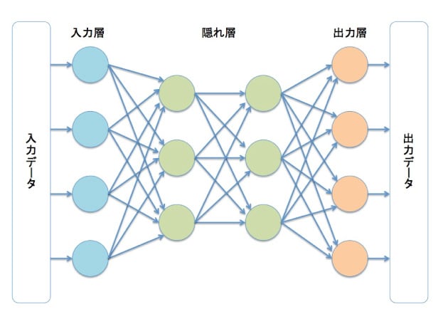
A neural network is similar to a function. However, it uses high-dimensional input values to output desired data. It can approximate very complex functions. A disadvantage is that it requires "learning" and lacks interpretability in its computation process.
x = [ x 1 , x 2 , . . . , x n ] ∈ R n \mathbf x=[x_1,x_2,...,x_n]\in\mathbb R^n x = [ x 1 , x 2 , ... , x n ] ∈ R n h i = f i ( W i h i − 1 + b i ) { f i : R m i − 1 → R m i ( activation function ) W i ∈ R m i × m i − 1 ( weight vector ) h i , b i ∈ R m i ( output and bias vector of layer i ) \mathbf h_i=f_i(\mathbf W_i\mathbf h_{i-1}+\mathbf b_i)\quad
\left\{
\begin{aligned}
f_i&:\mathbb R^{m_{i-1}}\to\mathbb R^{m_i}\quad(\text{activation function})\\
\mathbf W_i&\in\mathbb R^{m_i\times m_{i-1}}\quad(\text{weight vector})\\
\mathbf h_i,\mathbf b_i&\in\mathbb R^{m_i}\quad(\text{output and bias vector of layer } i)
\end{aligned}
\right. h i = f i ( W i h i − 1 + b i ) ⎩ ⎨ ⎧ f i W i h i , b i : R m i − 1 → R m i ( activation function ) ∈ R m i × m i − 1 ( weight vector ) ∈ R m i ( output and bias vector of layer i ) y = f o u t ( W o u t h l a s t + b o u t ) \mathbf y=f_{out}(\mathbf W_{out}\mathbf h_{last}+\mathbf b_{out}) y = f o u t ( W o u t h l a s t + b o u t ) y ^ = f N N ( x ; θ ) = f o u t ∘ f n ∘ f n − 1 ∘ . . . ∘ f 1 ( W 1 x + b 1 ) \hat{\mathbf y}=f_{NN}(x;\theta)=f_{out}\circ f_n\circ f_{n-1}\circ...\circ f_1(\mathbf W_1\mathbf x+\mathbf b_1) y ^ = f NN ( x ; θ ) = f o u t ∘ f n ∘ f n − 1 ∘ ... ∘ f 1 ( W 1 x + b 1 ) Here, ( \theta ) represents the parameters, including ( f ), ( W ), ( h ), and ( b ).
Activation functions introduce non-linearity.
f ( x ) = max ( 0 , x ) f(x)=\max(0,x) f ( x ) = max ( 0 , x ) f ( x ) = 1 1 + exp ( − x ) f(x)=\frac{1}{1+\exp(-x)} f ( x ) = 1 + exp ( − x ) 1 f ( x ) = tanh ( x ) = e x − e − x e x + e − x f(x)=\tanh(x)=\frac{e^x-e^{-x}}{e^x+e^{-x}} f ( x ) = tanh ( x ) = e x + e − x e x − e − x The integral of the sigmoid function:
f ( x ) = log ( 1 + exp ( x ) ) f(x)=\log(1+\exp(x)) f ( x ) = log ( 1 + exp ( x )) The calculation process from input to output:
y ^ = f N N ( x ; θ ) = f o u t ∘ f n ∘ f n − 1 ∘ . . . ∘ f 1 ( W 1 x + b 1 ) \hat{\mathbf y}=f_{NN}(x;\theta)=f_{out}\circ f_n\circ f_{n-1}\circ...\circ f_1(\mathbf W_1\mathbf x+\mathbf b_1) y ^ = f NN ( x ; θ ) = f o u t ∘ f n ∘ f n − 1 ∘ ... ∘ f 1 ( W 1 x + b 1 ) The process of calculating the error using a loss function based on the output and target data. Examples include Mean Squared Error (MSE) and Cross-Entropy Loss.
L = L o s s ( y , y ^ ) {\cal L}=Loss(\mathbf y,\hat{\mathbf y}) L = L oss ( y , y ^ ) The process of updating parameters based on the error using gradient descent.
W i ← W i − η ∂ L ∂ W i , b i ← b i − η ∂ L ∂ b i { ∂ L ∂ W i = ∂ L ∂ y ^ ⋅ ∂ y ^ ∂ h i ⋅ ∂ h i ∂ W i ∂ L ∂ b i = ∂ L ∂ y ^ ⋅ ∂ y ^ ∂ h i ⋅ ∂ h i ∂ b i \mathbf W_i\leftarrow\mathbf W_i-\eta\frac{\partial{\cal L}}{\partial\mathbf W_i},\quad\mathbf b_i\leftarrow\mathbf b_i-\eta\frac{\partial{\cal L}}{\partial\mathbf b_i}\quad
\left\{
\begin{aligned}
&\frac{\partial{\cal L}}{\partial\mathbf W_i}=\frac{\partial{\cal L}}{\partial\hat{\mathbf y}}\cdot\frac{\partial\hat{\mathbf y}}{\partial\mathbf h_i}\cdot\frac{\partial\mathbf h_i}{\partial\mathbf W_i}\\
&\frac{\partial{\cal L}}{\partial\mathbf b_i}=\frac{\partial{\cal L}}{\partial\hat{\mathbf y}}\cdot\frac{\partial\hat{\mathbf y}}{\partial\mathbf h_i}\cdot\frac{\partial\mathbf h_i}{\partial\mathbf b_i}
\end{aligned}
\right. W i ← W i − η ∂ W i ∂ L , b i ← b i − η ∂ b i ∂ L ⎩ ⎨ ⎧ ∂ W i ∂ L = ∂ y ^ ∂ L ⋅ ∂ h i ∂ y ^ ⋅ ∂ W i ∂ h i ∂ b i ∂ L = ∂ y ^ ∂ L ⋅ ∂ h i ∂ y ^ ⋅ ∂ b i ∂ h i This process ensures the gradients guide the parameters toward lower error values. It allows for efficient updates, especially when far from the minimum.
💡 The reason ( f'(x)=0 ) is not directly computed is that it is computationally difficult for computers. Instead, gradient descent is used since it is easier to compute the derivative numerically.
Why Use Gradient Descent in Machine Learning
θ t + 1 = θ t − η ∇ θ L ( θ t ) { θ t : parameters at time t η : learning rate ∇ θ L ( θ t ) : gradient of the loss function at time t \theta_{t+1}=\theta_t-\eta\nabla_\theta{\cal L}(\theta_t)
\left\{
\begin{aligned}
\theta_t:&\text{parameters at time } t\\
\eta:&\text{learning rate}\\
\nabla_\theta{\cal L}(\theta_t):&\text{gradient of the loss function at time } t
\end{aligned}
\right. θ t + 1 = θ t − η ∇ θ L ( θ t ) ⎩ ⎨ ⎧ θ t : η : ∇ θ L ( θ t ) : parameters at time t learning rate gradient of the loss function at time t Stop when ∣ ∣ ∇ θ ( θ t ) ∣ ∣ < ϵ ||\nabla_\theta{\cal}(\theta_t)||<\epsilon ∣∣ ∇ θ ( θ t ) ∣∣ < ϵ
Adam is more suited to deep learning, as it converges faster than standard gradient descent.
Compute the first moment: the moving average of the gradients (using exponential smoothing).
m t = β 1 m t − 1 + ( 1 − β 1 ) ∇ θ L ( θ t ) m_t=\beta_1m_{t-1}+(1-\beta_1)\nabla_\theta{\cal L}(\theta_t) m t = β 1 m t − 1 + ( 1 − β 1 ) ∇ θ L ( θ t )
Compute the second moment: the moving average of the squared gradients.
v t = β 2 v t − 1 + ( 1 − β 2 ) ( ∇ θ L ( θ t ) ) 2 v_t=\beta_2v_{t-1}+(1-\beta_2)(\nabla_\theta{\cal L}(\theta_t))^2 v t = β 2 v t − 1 + ( 1 − β 2 ) ( ∇ θ L ( θ t ) ) 2
Bias correction:
m ^ t = m t 1 − β 1 t , v ^ t = v t 1 − β 2 t \hat m_t=\frac{m_t}{1-\beta_1^t},~\hat v_t=\frac{v_t}{1-\beta_2^t} m ^ t = 1 − β 1 t m t , v ^ t = 1 − β 2 t v t
Update parameters:
θ t + 1 = θ t − η m ^ t v ^ t + ϵ \theta_{t+1}=\theta_t-\eta\frac{\hat m_t}{\sqrt{\hat v_t}+\epsilon} θ t + 1 = θ t − η v ^ t + ϵ m ^ t